Binary search tree
| Binary search tree | ||
|---|---|---|
| Type | Tree | |
| Invented | 1960 | |
| Invented by | P.F. Windley, A.D. Booth, A.J.T. Colin, and T.N. Hibbard | |
| Time complexity in big O notation | ||
| Average | Worst case | |
| Space | Θ(n) | O(n) |
| Search | Θ(log n) | O(n) |
| Insert | Θ(log n) | O(n) |
| Delete | Θ(log n) | O(n) |

In computer science, binary search trees (BST), sometimes called ordered or sorted binary trees, are a particular type of containers: data structures that store "items" (such as numbers, names etc.) in memory. They allow fast lookup, addition and removal of items, and can be used to implement either dynamic sets of items, or lookup tables that allow finding an item by its key (e.g., finding the phone number of a person by name).
Binary search trees keep their keys in sorted order, so that lookup and other operations can use the principle of binary search: when looking for a key in a tree (or a place to insert a new key), they traverse the tree from root to leaf, making comparisons to keys stored in the nodes of the tree and deciding, based on the comparison, to continue searching in the left or right subtrees. On average, this means that each comparison allows the operations to skip about half of the tree, so that each lookup, insertion or deletion takes time proportional to the logarithm of the number of items stored in the tree. This is much better than the linear time required to find items by key in an (unsorted) array, but slower than the corresponding operations on hash tables.
Several variants of the binary search tree have been studied in computer science; this article deals primarily with the basic type, making references to more advanced types when appropriate.
Definition
A binary search tree is a rooted binary tree, whose internal nodes each store a key (and optionally, an associated value) and each have two distinguished sub-trees, commonly denoted left and right. The tree additionally satisfies the binary search tree property, which states that the key in each node must be greater than all keys stored in the left sub-tree, and not greater than all keys in the right sub-tree.[1]:287 (The leaves (final nodes) of the tree contain no key and have no structure to distinguish them from one another. Leaves are commonly represented by a special leaf or nil symbol, a NULL pointer, etc.)
Generally, the information represented by each node is a record rather than a single data element. However, for sequencing purposes, nodes are compared according to their keys rather than any part of their associated records.
The major advantage of binary search trees over other data structures is that the related sorting algorithms and search algorithms such as in-order traversal can be very efficient; they are also easy to code.
Binary search trees are a fundamental data structure used to construct more abstract data structures such as sets, multisets, and associative arrays. Some of their disadvantages are as follows:
- The shape of the binary search tree depends entirely on the order of insertions and deletions, and can become degenerate.
- When inserting or searching for an element in a binary search tree, the key of each visited node has to be compared with the key of the element to be inserted or found.
- The keys in the binary search tree may be long and the run time may increase.
- After a long intermixed sequence of random insertion and deletion, the expected height of the tree approaches square root of the number of keys, √n, which grows much faster than log n.
Order relation
Binary search requires an order relation by which every element (item) can be compared with every other element in the sense of a total preorder. The part of the element which effectively takes place in the comparison is called its key. Whether duplicates, i.e. different elements with same key, shall be allowed in the tree or not, does not depend on the order relation, but on the application only.
In the context of binary search trees a total preorder is realized most flexibly by means of a three-way comparison subroutine.
Operations
Binary search trees support three main operations: insertion of elements, deletion of elements, and lookup (checking whether a key is present).
Searching
Searching a binary search tree for a specific key can be programmed recursively or iteratively.
We begin by examining the root node. If the tree is null, the key we are searching for does not exist in the tree. Otherwise, if the key equals that of the root, the search is successful and we return the node. If the key is less than that of the root, we search the left subtree. Similarly, if the key is greater than that of the root, we search the right subtree. This process is repeated until the key is found or the remaining subtree is null. If the searched key is not found after a null subtree is reached, then the key is not present in the tree. This is easily expressed as a recursive algorithm (implemented in Python):
1 def search_recursively(key, node):
2     if node is None or node.key == key:
3         return node
4     elif key < node.key:
5         return search_recursively(key, node.left)
6     else:  # key > node.key
7         return search_recursively(key, node.right)
The same algorithm can be implemented iteratively:
 1 def search_iteratively(key, node):
 2     current_node = node
 3     while current_node is not None:
 4         if key == current_node.key:
 5             return current_node
 6         elif key < current_node.key:
 7             current_node = current_node.left
 8         else:  # key > current_node.key:
 9             current_node = current_node.right
10     return None
These two examples rely on the order relation being a total order.
If the order relation is only a total preorder a reasonable extension of the functionality is the following: also in case of equality search down to the leaves in a direction specifiable by the user. A binary tree sort equipped with such a comparison function becomes stable.
Because in the worst case this algorithm must search from the root of the tree to the leaf farthest from the root, the search operation takes time proportional to the tree's height (see tree terminology). On average, binary search trees with n nodes have O(log n) height.[lower-alpha 1] However, in the worst case, binary search trees can have O(n) height, when the unbalanced tree resembles a linked list (degenerate tree).
Insertion
Insertion begins as a search would begin; if the key is not equal to that of the root, we search the left or right subtrees as before. Eventually, we will reach an external node and add the new key-value pair (here encoded as a record 'newNode') as its right or left child, depending on the node's key. In other words, we examine the root and recursively insert the new node to the left subtree if its key is less than that of the root, or the right subtree if its key is greater than or equal to the root.
Here's how a typical binary search tree insertion might be performed in a binary tree in C++:
Node* insert(Node*& root, int key, int value) {
  if (!root)
    root = new Node(key, value);
  else if (key < root->key)
    root->left = insert(root->left, key, value);
  else  // key >= root->key
    root->right = insert(root->right, key, value);
  return root;
}
The above destructive procedural variant modifies the tree in place. It uses only constant heap space (and the iterative version uses constant stack space as well), but the prior version of the tree is lost. Alternatively, as in the following Python example, we can reconstruct all ancestors of the inserted node; any reference to the original tree root remains valid, making the tree a persistent data structure:
 def binary_tree_insert(node, key, value):
     if node is None:
         return NodeTree(None, key, value, None)
     if key == node.key:
         return NodeTree(node.left, key, value, node.right)
     if key < node.key:
         return NodeTree(binary_tree_insert(node.left, key, value), node.key, node.value, node.right)
     else:
         return NodeTree(node.left, node.key, node.value, binary_tree_insert(node.right, key, value))
The part that is rebuilt uses O(log n) space in the average case and O(n) in the worst case.
In either version, this operation requires time proportional to the height of the tree in the worst case, which is O(log n) time in the average case over all trees, but O(n) time in the worst case.
Another way to explain insertion is that in order to insert a new node in the tree, its key is first compared with that of the root. If its key is less than the root's, it is then compared with the key of the root's left child. If its key is greater, it is compared with the root's right child. This process continues, until the new node is compared with a leaf node, and then it is added as this node's right or left child, depending on its key: if the key is less than the leaf's key, then it is inserted as the leaf's left child, otherwise as the leaf's right child.
There are other ways of inserting nodes into a binary tree, but this is the only way of inserting nodes at the leaves and at the same time preserving the BST structure.
Deletion
There are three possible cases to consider:
- Deleting a node with no children: simply remove the node from the tree.
- Deleting a node with one child: remove the node and replace it with its child.
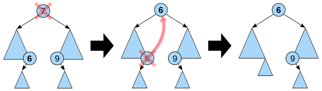
- Deleting a node with two children: call the node to be deleted N. Do not delete N. Instead, choose either its in-order successor node or its in-order predecessor node, R. Copy the value of R to N, then recursively call delete on the original R until reaching one of the first two cases. If you choose in-order successor of a node, as right sub tree is not NIL (Our present case is node has 2 children), then its in-order successor is node with least value in its right sub tree, which will have at a maximum of 1 sub tree, so deleting it would fall in one of the first 2 cases.
Broadly speaking, nodes with children are harder to delete. As with all binary trees, a node's in-order successor is its right subtree's left-most child, and a node's in-order predecessor is the left subtree's right-most child. In either case, this node will have zero or one children. Delete it according to one of the two simpler cases above.
Consistently using the in-order successor or the in-order predecessor for every instance of the two-child case can lead to an unbalanced tree, so some implementations select one or the other at different times.
Runtime analysis: Although this operation does not always traverse the tree down to a leaf, this is always a possibility; thus in the worst case it requires time proportional to the height of the tree. It does not require more even when the node has two children, since it still follows a single path and does not visit any node twice.
def find_min(self):   # Gets minimum node in a subtree
    current_node = self
    while current_node.left_child:
        current_node = current_node.left_child
    return current_node

def replace_node_in_parent(self, new_value=None):
    if self.parent:
        if self == self.parent.left_child:
            self.parent.left_child = new_value
        else:
            self.parent.right_child = new_value
    if new_value:
        new_value.parent = self.parent

def binary_tree_delete(self, key):
    if key < self.key:
        self.left_child.binary_tree_delete(key)
    elif key > self.key:
        self.right_child.binary_tree_delete(key)
    else: # delete the key here
        if self.left_child and self.right_child: # if both children are present
            successor = self.right_child.find_min()
            self.key = successor.key
            successor.binary_tree_delete(successor.key)
        elif self.left_child:   # if the node has only a *left* child
            self.replace_node_in_parent(self.left_child)
        elif self.right_child:  # if the node has only a *right* child
            self.replace_node_in_parent(self.right_child)
        else: # this node has no children
            self.replace_node_in_parent(None)
Traversal
Once the binary search tree has been created, its elements can be retrieved in-order by recursively traversing the left subtree of the root node, accessing the node itself, then recursively traversing the right subtree of the node, continuing this pattern with each node in the tree as it's recursively accessed. As with all binary trees, one may conduct a pre-order traversal or a post-order traversal, but neither are likely to be useful for binary search trees. An in-order traversal of a binary search tree will always result in a sorted list of node items (numbers, strings or other comparable items).
The code for in-order traversal in Python is given below. It will call callback (some function the programmer wishes to call on the node's value, such as printing to the screen) for every node in the tree.
def traverse_binary_tree(node, callback):
    if node is None:
        return
    traverse_binary_tree(node.leftChild, callback)
    callback(node.value)
    traverse_binary_tree(node.rightChild, callback)
Traversal requires O(n) time, since it must visit every node. This algorithm is also O(n), so it is asymptotically optimal.
Traversal can also be implemented iteratively. For certain applications, e.g. greater equal search, approximative search, an operation for single step (iterative) traversal can be very useful. This is, of course, implemented without the callback construct and takes O(1) on average and O(log n) in the worst case.
Verification
Sometimes we already have a binary tree, and we need to determine whether it is a BST. This problem has a simple recursive solution.
The BST property—every node on the right subtree has to be larger than the current node and every node on the left subtree has to be smaller than (or equal to - should not be the case as only unique values should be in the tree - this also poses the question as to if such nodes should be left or right of this parent) the current node—is the key to figuring out whether a tree is a BST or not. The greedy algorithm – simply traverse the tree, at every node check whether the node contains a value larger than the value at the left child and smaller than the value on the right child – does not work for all cases. Consider the following tree:
     20
    /  \
  10    30
       /  \
      5    40
In the tree above, each node meets the condition that the node contains a value larger than its left child and smaller than its right child hold, and yet it is not a BST: the value 5 is on the right subtree of the node containing 20, a violation of the BST property.
Instead of making a decision based solely on the values of a node and its children, we also need information flowing down from the parent as well. In the case of the tree above, if we could remember about the node containing the value 20, we would see that the node with value 5 is violating the BST property contract.
So the condition we need to check at each node is:
- if the node is the left child of its parent, then it must be smaller than (or equal to) the parent and it must pass down the value from its parent to its right subtree to make sure none of the nodes in that subtree is greater than the parent
- if the node is the right child of its parent, then it must be larger than the parent and it must pass down the value from its parent to its left subtree to make sure none of the nodes in that subtree is lesser than the parent.
A recursive solution in C++ can explain this further:
struct TreeNode {
    int key;
    int value;
    struct TreeNode *left;
    struct TreeNode *right;
};

bool isBST(struct TreeNode *node, int minKey, int maxKey) {
    if(node == NULL) return true;
    if(node->key < minKey || node->key > maxKey) return false;

    return isBST(node->left, minKey, node->key) && isBST(node->right, node->key, maxKey);
}
The initial call to this function can be something like this:
if(isBST(root, INT_MIN, INT_MAX)) {
    puts("This is a BST.");
} else {
    puts("This is NOT a BST!");
}
Essentially we keep creating a valid range (starting from [MIN_VALUE, MAX_VALUE]) and keep shrinking it down for each node as we go down recursively.
As pointed out in section #Traversal, an in-order traversal of a binary search tree returns the nodes sorted. Thus we only need to keep the last visited node while traversing the tree and check whether its key is smaller (or smaller/equal, if duplicates are to be allowed in the tree) compared to the current key.
Examples of applications
Some examples shall illustrate the use of above basic building blocks.
Sort
A binary search tree can be used to implement a simple sorting algorithm. Similar to heapsort, we insert all the values we wish to sort into a new ordered data structure—in this case a binary search tree—and then traverse it in order.
The worst-case time of build_binary_tree is O(n2)—if you feed it a sorted list of values, it chains them into a linked list with no left subtrees. For example, build_binary_tree([1, 2, 3, 4, 5]) yields the tree (1 (2 (3 (4 (5))))).
There are several schemes for overcoming this flaw with simple binary trees; the most common is the self-balancing binary search tree. If this same procedure is done using such a tree, the overall worst-case time is O(n log n), which is asymptotically optimal for a comparison sort. In practice, the added overhead in time and space for a tree-based sort (particularly for node allocation) make it inferior to other asymptotically optimal sorts such as heapsort for static list sorting. On the other hand, it is one of the most efficient methods of incremental sorting, adding items to a list over time while keeping the list sorted at all times.
Priority queue operations
Binary search trees can serve as priority queues: structures that allow insertion of arbitrary key as well as lookup and deletion of the minimum (or maximum) key. Insertion works as previously explained. Find-min walks the tree, following left pointers as far as it can without hitting a leaf:
// Precondition: T is not a leaf
function find-min(T):
    while hasLeft(T):
        T ? left(T)
    return key(T)
Find-max is analogous: follow right pointers as far as possible. Delete-min (max) can simply look up the minimum (maximum), then delete it. This way, insertion and deletion both take logarithmic time, just as they do in a binary heap, but unlike a binary heap and most other priority queue implementations, a single tree can support all of find-min, find-max, delete-min and delete-max at the same time, making binary search trees suitable as double-ended priority queues.[2]:156
Types
There are many types of binary search trees. AVL trees and red-black trees are both forms of self-balancing binary search trees. A splay tree is a binary search tree that automatically moves frequently accessed elements nearer to the root. In a treap (tree heap), each node also holds a (randomly chosen) priority and the parent node has higher priority than its children. Tango trees are trees optimized for fast searches. T-trees are binary search trees optimized to reduce storage space overhead, widely used for in-memory databases
A degenerate tree is a tree where for each parent node, there is only one associated child node. It is unbalanced and, in the worst case, performance degrades to that of a linked list. If your added node function does not handle re-balancing, then you can easily construct a degenerate tree by feeding it with data that is already sorted. What this means is that in a performance measurement, the tree will essentially behave like a linked list data structure.
Performance comparisons
D. A. Heger (2004)[3] presented a performance comparison of binary search trees. Treap was found to have the best average performance, while red-black tree was found to have the smallest amount of performance variations.
Optimal binary search trees
If we do not plan on modifying a search tree, and we know exactly how often each item will be accessed, we can construct[4] an optimal binary search tree, which is a search tree where the average cost of looking up an item (the expected search cost) is minimized.
Even if we only have estimates of the search costs, such a system can considerably speed up lookups on average. For example, if you have a BST of English words used in a spell checker, you might balance the tree based on word frequency in text corpora, placing words like the near the root and words like agerasia near the leaves. Such a tree might be compared with Huffman trees, which similarly seek to place frequently used items near the root in order to produce a dense information encoding; however, Huffman trees store data elements only in leaves, and these elements need not be ordered.
If we do not know the sequence in which the elements in the tree will be accessed in advance, we can use splay trees which are asymptotically as good as any static search tree we can construct for any particular sequence of lookup operations.
Alphabetic trees are Huffman trees with the additional constraint on order, or, equivalently, search trees with the modification that all elements are stored in the leaves. Faster algorithms exist for optimal alphabetic binary trees (OABTs).
See also
Notes
- ↑ The notion of an average BST is made precise as follows. Let a random BST be one built using only insertions out of a sequence of unique elements in random order (all permutations equally likely); then the expected height of the tree is O(log n). If deletions are allowed as well as insertions, "little is known about the average height of a binary search tree".[1]:300
References
- 1 2 Cormen, Thomas H.; Leiserson, Charles E.; Rivest, Ronald L.; Stein, Clifford (2009) [1990]. Introduction to Algorithms (3rd ed.). MIT Press and McGraw-Hill. ISBN 0-262-03384-4.
- ↑ Mehlhorn, Kurt; Sanders, Peter (2008). Algorithms and Data Structures: The Basic Toolbox (PDF). Springer.
- ↑ Heger, Dominique A. (2004), "A Disquisition on The Performance Behavior of Binary Search Tree Data Structures" (PDF), European Journal for the Informatics Professional, 5 (5): 67–75
- ↑ Gonnet, Gaston. "Optimal Binary Search Trees". Scientific Computation. ETH Zürich. Retrieved 1 December 2013.
Further reading
 This article incorporates public domain material from the NIST document: Black, Paul E. "Binary Search Tree". Dictionary of Algorithms and Data Structures.
- Cormen, Thomas H.; Leiserson, Charles E.; Rivest, Ronald L.; Stein, Clifford (2001). "12: Binary search trees, 15.5: Optimal binary search trees". Introduction to Algorithms (2nd ed.). MIT Press & McGraw-Hill. pp. 253–272, 356–363. ISBN 0-262-03293-7.
- Jarc, Duane J. (3 December 2005). "Binary Tree Traversals". Interactive Data Structure Visualizations. University of Maryland.
- Knuth, Donald (1997). "6.2.2: Binary Tree Searching". The Art of Computer Programming. 3: "Sorting and Searching" (3rd ed.). Addison-Wesley. pp. 426–458. ISBN 0-201-89685-0.
- Long, Sean. "Binary Search Tree" (PPT). Data Structures and Algorithms Visualization-A PowerPoint Slides Based Approach. SUNY Oneonta.
- Parlante, Nick (2001). "Binary Trees". CS Education Library. Stanford University.
External links
- Literate implementations of binary search trees in various languages on LiteratePrograms
- Binary Tree Visualizer (JavaScript animation of various BT-based data structures)
- Kovac, Kubo. "Binary Search Trees" (Java applet). Korešponden?ný seminár z programovania.
- Madru, Justin (18 August 2009). "Binary Search Tree". JDServer. C++ implementation.
- Binary Search Tree Example in Python
- "References to Pointers (C++)". MSDN. Microsoft. 2005. Gives an example binary tree implementation.