Brooks–Iyengar algorithm
The Brooks–Iyengar algorithm or Brooks–Iyengar hybrid algorithm [1] is a distributed algorithm, that improves both the precision and accuracy of the interval measurements taken by a distributed sensor network, even in the presence of faulty sensors.[2] The sensor network does this by exchanging the measured value and accuracy value at every node with every other node. And it computes the accuracy range and a measured value for the whole network from all of the values collected. Even if some of the data from some of the sensors is faulty, the sensor network will not malfunction. The algorithm is fault-tolerant and distributed. It could also be used as a sensor fusion method. The precision and accuracy bound of this algorithm have been proved in 2016.[3]
Background
The Brooks–Iyengar hybrid algorithm for distributed control in the presence of noisy data combines Byzantine agreement with sensor fusion. It bridges the gap between sensor fusion and Byzantine fault tolerance.[4] This seminal algorithm unified these disparate fields for the first time. Essentially, it combines Dolev’s[5] algorithm for approximate agreement with Mahaney and Schneider’s fast convergence algorithm (FCA). The algorithm assumes N processing elements (PEs), t of which are faulty and can behave maliciously. It takes as input either real values with inherent inaccuracy or noise (which can be unknown), or a real value with apriori defined uncertainty, or an interval. The output of the algorithm is a real value with an explicitly specified accuracy. The algorithm runs in O(NlogN) where N is the number of PEs: see Big O notation. It is possible to modify this algorithm to correspond to Crusader’s Convergence Algorithm (CCA),[6] however, the bandwidth requirement will also increase. The algorithm has applications in distributed control, software reliability, High-performance computing, etc.[7]
Algorithm
The Brooks–Iyengar algorithm is executed in every sensor node of a distributed sensor network. Each sensor exchanges their measured value and accuracy value with all other sensors in the network. The accuracy range the algorithm finds is the lowest lower bound and the highest upper bound returned from all the sensors. The "fused" measurement is a weighted average of the midpoints of the regions found.[8] The concrete steps of Brooks-Iyengar algorithm are shown in this section. Each PE performs the estimation separately:
Input:
The measurement sent by PE k to PE i is a closed interval ,
![{\displaystyle [l_{k,i},h_{k,i}]}](../I/m/1bdd207089aac564b9ddf02e283e0b54c179a336.svg)

Output:
The output of PE i includes a point estimate and an interval estimate
- PE i receives measurements from all the other PEs.
- Divide the union of collected measurements into mutually exclusive intervals based on the number of measurements that intersect, which is known as the weight of the interval.
- Remove intervals with weight less than , where is the number of faulty PEs
- If there are L intervals left, let denote the set of the remaining intervals. We have , where interval and is the weight associated with interval . We also assume .
- Calculate the point estimate of PE i as and the interval estimate is


![{\displaystyle I_{l}^{i}=[l_{I_{l}^{i}},h_{I_{l}^{i}}]}](../I/m/a0d9d7d4334b43abe9910fac26f4c51326e18086.svg)


![{\displaystyle [l_{I_{1}^{i}},h_{I_{L}^{i}}]}](../I/m/f33cbf9b12ba1b55366888a8554ca7aed6fd5e5b.svg)
Example:
Consider an example of 5 PEs, in which PE 5 () is sending wrong values to other PEs. The following Table is the values received by .


| values |


![{\displaystyle [2.7,6.7]}](../I/m/cc082c8d1124565970c95c32080ef875b635edfd.svg)
![{\displaystyle [0,3.2]}](../I/m/12d3dfa4bf1326e41682e271580ce13cdf905024.svg)
![{\displaystyle [1.5,4.5]}](../I/m/a1252e11c8e9dad706c264ff9a7f2fdb19f35c0e.svg)
![{\displaystyle [0.8,2.8]}](../I/m/649a5d6da7327c464a36ba9ff300cc4672303ef2.svg)
![{\displaystyle [1.4,4.6]}](../I/m/5cddd3d1e6a7f98d8e90776ded5e83959f6471b7.svg)
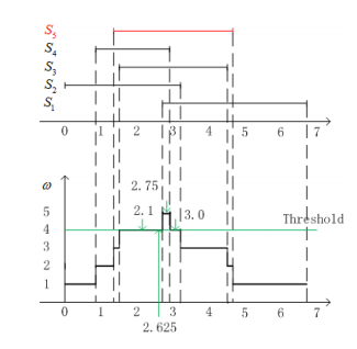
We draw a Weighted Region Diagram (WRD) of these intervals, then we can determine for PE 1 according to the Algorithm:

![{\displaystyle A_{1}=\{([1.5,2.7],4),([2.7,2.8],5),([2.8,3.2],4)\}}](../I/m/58b4d0f0f1a1366b3147818d04c7437eafea350a.svg)
which consists of intervals where at least 4(= = 5−1) measurements intersect. The output of PE 1 is equal to

and the interval estimate is
![{\displaystyle [1.5,3.2]}](../I/m/22ffab057d8d796da4de7ab039824f9737badbde.svg)
Algorithm characteristics
- Faulty PEs tolerated < N/3
- Maximum faulty PEs < 2N/3
- Complexity = O(N log N)
- Order of network bandwidth = O(N)
- Convergence = 2t/N
- Accuracy = limited by input
- Iterates for precision = often
- Precision over accuracy = no
- Accuracy over precision = no
See also
- Distributed sensor network
- Sensor fusion
- Fault tolerance
- Consensus (computer science)
- Consensus algorithm
- Paxos (computer science)
- Raft (computer science)
- Marzullo's algorithm
- Intersection algorithm
References
- ↑ Richard R. Brooks & S. Sithrama Iyengar (June 1996). "Robust Distributed Computing and Sensing Algorithm". Computer. IEEE. 29 (6): 53–60. doi:10.1109/2.507632. ISSN 0018-9162. Retrieved 2010-03-22.
- ↑ Mohammad Ilyas; Imad Mahgoub (July 28, 2004). Handbook of sensor networks: compact wireless and wired sensing systems (PDF). bit.csc.lsu.edu. CRC Press. pp. 25–4, 33–2 of 864. ISBN 978-0-8493-1968-6. Retrieved 2010-03-22.
- ↑ "On Precision Bound of Distributed Fault-Tolerant Sensor Fusion Algorithms". ACM Computing Surveys (CSUR). 49 (1, July 2016).
- ↑ D. Dolev (Jan 1982). "The Byzantine Generals Strike Again" (PDF). J. Algorithms. 3 (1): 14–30. doi:10.1016/0196-6774(82)90004-9. Retrieved 2010-03-22.
- ↑ L. Lamport; R. Shostak; M. Pease (July 1982). "The Byzantine Generals Problem". Transactions on Programming Languages and Systems. ACM. 4 (3): 382–401. doi:10.1145/357172.357176. Retrieved 2010-03-22.
- ↑ D. Dolev; et al. (July 1986). "Reaching Approximate Agreement in the Presence of Faults" (PDF). Journal of the ACM (JACM). ACM Press. 33 (3): 499–516. doi:10.1145/5925.5931. ISSN 0004-5411. Retrieved 2010-03-23.
- ↑ S. Mahaney & F. Schneider (1985). "Inexact Agreement: Accuracy, Precision, and Graceful Degradation". Proc. Fourth ACM Symp. Principles of Distributed Computing. ACM Press, New York,: 237–249. CiteSeerX 10.1.1.20.6337
 .
. - ↑ Sartaj Sahni and Xiaochun Xu (September 7, 2004). "Algorithms For Wireless Sensor Networks" (PDF). University of Florida, Gainesville. Retrieved 2010-03-23.