Dirichlet eta function

For the modular form, see Dedekind eta function.

Color representation of the Dirichlet eta function. It is generated as a Matplotlib plot using a version of the Domain coloring method.^[1]

In mathematics, in the area of analytic number theory, the Dirichlet eta function is defined by the following Dirichlet series, which converges for any complex number having real part > 0:

\eta(s) = \sum_{n=1}^{\infty}{(-1)^{n-1} \over n^s} = \frac{1}{1^s} - \frac{1}{2^s} + \frac{1}{3^s} - \frac{1}{4^s} + \cdots

This Dirichlet series is the alternating sum corresponding to the Dirichlet series expansion of the Riemann zeta function, ζ(s) — and for this reason the Dirichlet eta function is also known as the alternating zeta function, also denoted ζ*(s). The following relation holds:

\eta(s) = \left(1-2^{1-s}\right) \zeta(s)

While the Dirichlet series expansion for the eta function is convergent only for any complex number s with real part > 0, it is Abel summable for any complex number. This serves to define the eta function as an entire function (and the above relation then shows the zeta function is meromorphic with a simple pole at s = 1, and perhaps poles at the other zeros of the factor $1-2^{1-s}$ ).

Equivalently, we may begin by defining

\eta(s) = \frac{1}{\Gamma(s)}\int_0^\infty \frac{x^{s-1}}{e^x+1}{dx}

which is also defined in the region of positive real part ( $\Gamma(s)$ represents the Gamma function). This gives the eta function as a Mellin transform.

Hardy gave a simple proof of the functional equation for the eta function, which is

\eta(-s) = 2 \frac{1-2^{-s-1}}{1-2^{-s}} \pi^{-s-1} s \sin\left({\pi s \over 2}\right) \Gamma(s)\eta(s+1).

From this, one immediately has the functional equation of the zeta function also, as well as another means to extend the definition of eta to the entire complex plane.

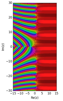
Zeros

The zeros of the eta function include all the zeros of the zeta function: the infinity of negative even integers (real equidistant simple zeros); an infinity of zeros along the critical line, none of which are known to be multiple and over 40% of which have been proven to be simple, and the hypothetical zeros in the critical strip but not on the critical line, which if they do exist must occur at the vertices of rectangles symmetrical around the x-axis and the critical line and whose multiplicity is unknown. In addition, the factor $1-2^{1-s}$ adds an infinity of complex simple zeros, located at equidistant points on the line $\Re(s)=1$ , at $s_n=1+2n\pi i/\log(2)$ where n is any nonzero integer.

Under the Riemann hypothesis, the zeros of the eta function would be located symmetrically with respect to the real axis on two parallel lines $\Re(s)=1/2, \Re(s)=1$ , and on the perpendicular half line formed by the negative real axis.

Landau's problem with ζ(s) = η(s)/0 and solutions

In the equation η(s) = (1−2^1−s) ζ(s), "the pole of ζ(s) at s=1 is cancelled by the zero of the other factor" (Titchmarsh, 1986, p. 17), and as a result η(1) is neither infinite nor zero. However, in the equation

\zeta(s)=\frac{\eta(s)}{1-2^{1-s}},

η must be zero at all the points $s_n = 1+n\frac{2\pi}{\ln{2}}i, n\ne0, n \in Z$ , where the denominator is zero, if the Riemann zeta function is analytic and finite there. The problem of proving this without defining the zeta function first was signaled and left open by E. Landau in his 1909 treatise on number theory: "Whether the eta series is different from zero or not at the points $s_n\ne1$ , i.e., whether these are poles of zeta or not, is not readily apparent here."

A first solution for Landau's problem was published almost 40 years later by D. V. Widder in his book The Laplace Transform. It uses the next prime 3 instead of 2 to define a Dirichlet series similar to the eta function, which we will call the $\lambda$ function, defined for $\Re (s)>0$ and with some zeros also on $\Re(s)=1$ , but not equal to those of eta.

Indirect proof of eta(s_n) = 0 following Widder

\begin{align} \lambda(s)=(1-\frac{3}{3^s})\zeta(s) = (1+\frac{1}{2^s})-\frac{2}{3^s}+(\frac{1}{4^s}+\frac{1}{5^s})-\frac{2}{6^s}+\ldots \end{align}

If $s$ is real and strictly positive, the series converges since the regrouped terms alternate in sign and decrease in absolute value to zero. According to a theorem on uniform convergence of Dirichlet series first proven by Cahen in 1894, the $\lambda(s)$ function is then analytic for $\Re (s)>0$ , a region which includes the line $\Re(s)=1$ . Now we can define correctly, where the denominators are not zero,

\zeta(s) = \frac{\eta(s)}{1-\frac{2}{2^s}}

\zeta(s) = \frac{\lambda(s)}{1-\frac{3}{3^s}}

Since $\frac{\log 3}{\log 2}$ is irrational, the denominators in the two definitions are not zero at the same time except for $s=1$ , and the $\zeta(s)\,$ function is thus well defined and analytic for $\Re (s)>0$ except at $s=1$ . We finally get indirectly that $\eta(s_n)=0$ when $s_n\ne1$ :

\eta(s_n) = (1-\frac{2}{2^{s_n}})\zeta(s_n) = \frac{1-\frac{2}{2^{s_n}}}{1-\frac{3}{3^{s_n}}} \lambda(s_n) = 0.

An elementary direct and $\zeta\,$ -independent proof of the vanishing of the eta function at $s_n\ne1$ was published by J. Sondow in 2003. It expresses the value of the eta function as the limit of special Riemann sums associated to an integral known to be zero, using a relation between the partial sums of the Dirichlet series defining the eta and zeta functions for $\Re(s)>1$ .

Direct proof of eta(s_n) = 0 by Sondow

With some simple algebra performed on finite sums, we can write for any complex s

\eta_{2n}(s) = \sum_{k=1}^{2n}\frac{(-1)^{k-1}}{k^s} = 1-\frac{1}{2^s}+\frac{1}{3^s}-\frac{1}{4^s}+\ldots+\frac{(-1)^{2n-1}}{{(2n)}^s} = 1+\frac{1}{2^s}+\frac{1}{3^s}+\frac{1}{4^s}+\ldots+\frac{1}{{(2n)}^s} - 2(\frac{1}{2^s}+\frac{1}{4^s}+\ldots+\frac{1}{{(2n)}^s})

= (1-\frac{2}{2^s})\zeta_{2n}(s) + \frac{2}{2^s}(\frac{1}{{(n+1)}^s}+\ldots+\frac{1}{{(2n)}^s}) = (1-\frac{2}{2^s})\zeta_{2n}(s) + \frac{2n}{{(2n)}^s}\,\frac{1}{n}\,(\frac{1}{{(1+1/n)}^s}+ \ldots + \frac{1}{{(1+n/n)}^s}).

Now if $s=1+it$ and $2^s=2$ , the factor multiplying $\zeta_{2n}(s)\,$ is zero, and

\eta_{2n}(s) = \frac{1}{n^{it}} R_n(\frac{1}{{(1+x)}^s},0,1),

where Rn(f(x),a,b) denotes a special Riemann sum approximating the integral of f(x) over [a,b]. For t = 0 i.e. s = 1, we get

\eta(1) = \lim_{n\to\infty} \eta_{2n}(1) = \lim_{n\to\infty} R_n(\frac{1}{1+x},0,1) = \int_0^1 \frac{dx}{1+x} = \log 2 \ne 0.

Otherwise, if $t\ne0$ , then $|n^{1-s}|=|n^{-it}|=1$ , which yields

|\eta(s)| = \lim_{n\to\infty} |\eta_{2n}(s)| = \lim_{n\to\infty} |R_n(\frac{1}{{(1+x)}^s},0,1)| = |\int_0^1 \frac{dx}{{(1+x)}^s}| = |\frac{2^{1-s}-1}{1-s}| = |\frac{1-1}{-it}| = 0.

Assuming $\eta(s_n)=0$ , for each point $s_n\ne1$ where $2^{s_n}=2$ , we can now define $\zeta(s_n)\,$ by continuity as follows,

\zeta(s_n) = \lim_{s\to s_n}\frac{\eta(s)}{1-\frac{2}{2^s}} = \lim_{s\to s_n}\frac{\eta(s)-\eta(s_n)}{\frac{2}{2^{s_n}}-\frac{2}{2^s}} = \lim_{s\to s_n}\frac{\eta(s)-\eta(s_n)}{s-s_n}\,\frac{s-s_n}{\frac{2}{2^{s_n}}-\frac{2}{2^s}} = \frac{\eta'(s_n)}{\log(2)}.

The apparent singularity of zeta at $s_n\ne1$ is now removed, and the zeta function is proven to be analytic everywhere in $\Re{s} > 0$ , except at $s=1$ where

\lim_{s\to1} (s-1)\zeta(s) = \lim_{s\to 1} \frac{\eta(s)}{\frac{1-2^{1-s}}{s-1}} = \frac{\eta(1)}{\log 2} = 1.

Integral representations

A number of integral formulas involving the eta function can be listed. The first one follows from a change of variable of the integral representation of the Gamma function (Abel, 1823), giving a Mellin transform which can be expressed in different ways as a double integral (Sondow, 2005). This is valid for $\Re s > 0.$

\begin{align} \Gamma(s)\eta(s) & = \int_0^\infty \frac{x^{s-1}}{e^x+1} \, dx = \int_0^\infty \int_0^x \frac{x^{s-2}}{e^x+1} \, dy \, dx \\[8pt] & =\int_0^\infty\int_0^\infty \frac{(t+r)^{s-2}}{e^{t+r}+1}{dr} \, dt =\int_0^1\int_0^1 \frac{(-\log(x y))^{s-2}}{1 + x y} \, dx \, dy. \end{align}

The Cauchy–Schlömilch transformation (Amdeberhan, Moll et al., 2010) can be used to prove this other representation, valid for $\Re s > -1$ . Integration by parts of the first integral above in this section yields another derivation.

2^{1-s}\,\Gamma(s+1)\,\eta(s) = 2 \int_0^\infty \frac{x^{2s+1}}{\cosh^2(x^2)} \, dx = \int_0^\infty \frac{t^s}{\cosh^2(t)} \, dt.

The next formula, due to Lindelöf (1905), is valid over the whole complex plane, when the principal value is taken for the logarithm implicit in the exponential.

\eta(s) = \int_{-\infty}^\infty \frac{(1/2 + i t)^{-s}}{e^{\pi t}+e^{-\pi t}} \, dt.

This corresponds to a Jensen (1895) formula for the entire function $(s-1)\,\zeta(s)$ , valid over the whole complex plane and also proven by Lindelöf.

(s-1)\zeta (s)=2\pi \,\int _{{-\infty }}^{\infty }{\frac {(1/2+it)^{{1-s}}}{(e^{{\pi t}}+e^{{-\pi t}})^{2}}}\,dt.

"This formula, remarquable by its simplicity, can be proven easily with the help of Cauchy's theorem, so important for the summation of series" wrote Jensen (1895). Similarly by converting the integration paths to contour integrals one can obtain other formulas for the eta function, such as this generalisation (Milgram, 2013) valid for $0<c< 1$ and all $s$ :

\eta(s) = \frac{1}{2} \int_{-\infty}^\infty \frac{(c + i t)^{-s}}{\sin{(\pi(c+i t))}} \, dt.

The zeros on the negative real axis are factored out cleanly by making $c\to 0^+$ (Milgram, 2013) to obtain a formula valid for $\Re s < 0$ :

\eta (s)=-\sin \left({\frac {s\pi }{2}}\right)\int _{{0}}^{\infty }{\frac {t^{{-s}}}{\sinh {(\pi t)}}}\,dt.

Numerical algorithms

Most of the series acceleration techniques developed for alternating series can be profitably applied to the evaluation of the eta function. One particularly simple, yet reasonable method is to apply Euler's transformation of alternating series, to obtain

\eta(s)=\sum_{n=0}^\infty \frac{1}{2^{n+1}} \sum_{k=0}^n (-1)^{k} {n \choose k} \frac {1}{(k+1)^s}.

Note that the second, inside summation is a forward difference.

Borwein's method

Peter Borwein used approximations involving Chebyshev polynomials to produce a method for efficient evaluation of the eta function. If

d_k = n\sum_{i=0}^k \frac{(n+i-1)!4^i}{(n-i)!(2i)!}

then

\eta(s) = -\frac{1}{d_n} \sum_{k=0}^{n-1}\frac{(-1)^k(d_k-d_n)}{(k+1)^s}+\gamma_n(s),

where for $\Re(s) \ge \frac{1}{2}$ the error term γ_n is bounded by

|\gamma_n(s)| \le \frac{3}{(3+\sqrt{8})^n} (1+2|\Im(s)|)\exp(\frac{\pi}{2}|\Im(s)|).

The factor of $3+\sqrt{8}\approx 5.8$ in the error bound indicates that the Borwein series converges quite rapidly as n increases.

Particular values

Further information: Zeta constant

η(0) = ¹⁄₂, the Abel sum of Grandi's series 1 − 1 + 1 − 1 + · · ·.
η(−1) = ¹⁄₄, the Abel sum of 1 − 2 + 3 − 4 + · · ·.
For k an integer > 1, if B_k is the k-th Bernoulli number then
$\eta(1-k) = \frac{2^k-1}{k} B_k.$

Also:

\!\ \eta(1) = \ln2

, this is the alternating harmonic series

\eta(2) = {\pi^2 \over 12}

A072691

\eta(4) = {{7\pi^4} \over 720} \approx 0.94703283

\eta(6) = {{31\pi^6} \over 30240} \approx 0.98555109

\eta(8) = {{127\pi^8} \over 1209600} \approx 0.99623300

\eta(10) = {{73\pi^{10}} \over 6842880} \approx 0.99903951

\eta(12) = {{1414477\pi^{12}} \over {1307674368000}} \approx 0.99975769

The general form for even positive integers is:

$\eta(2n) = (-1)^{n+1}{{B_{2n}\pi^{2n}(2^{2n-1} - 1)} \over {(2n)!}}.$

Derivatives

The derivative with respect to the parameter $s$ is for $s\neq 1$

\eta'(s) = \sum_{n=1}^\infty \frac{(-1)^n\ln n}{n^s} = 2^{1-s}\ln 2 \zeta(s)+(1-2^{1-s})\zeta'(s)

\eta'(1) = \ln(2)\gamma-\ln(2)^2/2

References

↑ http://nbviewer.ipython.org/github/empet/Math/blob/master/DomainColoring.ipynb

Jensen, J. L. W. V. (1895). L'Intermédiaire des Mathématiciens. II: 346. Missing or empty |title= (help)
Lindelöf, Ernst (1905). Le calcul des résidus et ses applications à la théorie des fonctions. Gauthier-Villars. p. 103.
Widder, David Vernon (1946). The Laplace Transform. Princeton University Press. p. 230.
Landau, Edmund, Handbuch der Lehre von der Verteilung der Primzahlen, Erster Band, Berlin, 1909, p. 160. (Second edition by Chelsea, New York, 1953, p. 160, 933)
Titchmarsh, E. C. (1986). The Theory of the Riemann Zeta Function, Second revised (Heath-Brown) edition. Oxford University Press.
Conrey, J. B. (1989). "More than two fifths of the zeros of the Riemann zeta function are on the critical line". Journal für die Reine und Angewandte Mathematik. 399: 1–26. doi:10.1515/crll.1989.399.1.
Knopp, Konrad (1990) [1922]. Theory and Application of Infinite Series. Dover. ISBN 0-486-66165-2.
Borwein, P., An Efficient Algorithm for the Riemann Zeta Function, Constructive experimental and nonlinear analysis, CMS Conference Proc. 27 (2000), 29–34.
Sondow, Jonathan (2002). "Double integrals for Euler's constant and ln 4/π and an analog of Hadjicostas's formula". arXiv:math.CO/0211148. Amer. Math. Monthly 112 (2005) 61–65, formula 18.
Sondow, Jonathan. "Zeros of the Alternating Zeta Function on the Line R(s)=1". arXiv:math/0209393. Amer. Math. Monthly, 110 (2003) 435–437.
Gourdon, Xavier; Sebah, Pascal (2003). "Numerical evaluation of the Riemann Zeta-function" (PDF).
Amdeberhan, T.; Glasser, M. L.; Jones, M. C; Moll, V. H.; Posey, R.; Varela, D. (2010). "The Cauchy–Schlomilch Transformation". arXiv:1004.2445. p. 12.
Milgram, Michael S. (2012). "Integral and Series Representations of Riemann's Zeta Function, Dirichlet's Eta Function and a Medley of Related Results". arXiv:1208.3429. . Journal of Mathematics (2013) doi:10.1155/2013/181724.

This article is issued from Wikipedia - version of the 7/24/2016. The text is available under the Creative Commons Attribution/Share Alike but additional terms may apply for the media files.