Proxmap sort
 Example of insertion sort sorting a list of random numbers. | |
| Class | Sorting algorithm |
|---|---|
| Data structure | Array |
| Worst-case performance | |
| Best-case performance | |
| Average performance | |
| Worst-case space complexity | |


ProxmapSort, or Proxmap sort, is a sorting algorithm that works by partitioning an array of data items, or keys, into a number of "subarrays" (termed buckets, in similar sorts). The name is short for computing a "proximity map," which indicates for each key K the beginning of a subarray where K will reside in the final sorted order. Keys are placed into each subarray using insertion sort. If keys are "well distributed" among the subarrays, sorting occurs in linear time. The computational complexity estimates involve the number of subarrays and the proximity mapping function, the "map key," used. It is a form of bucket and radix sort.
Once a ProxmapSort is complete, ProxmapSearch can be used to find keys in the sorted array in time if the keys were well distributed during the sort.

Both algorithms were invented in the late 1980s by Prof. Thomas A. Standish at the University of California, Irvine.
Overview
Basic strategy
In general: Given an array A with n keys:
- map a key to a subarray of the destination array A2, by applying the map key function to each array item
- determine how many keys will map to the same subarray, using an array of "hit counts," H
- determine where each subarray will begin in the destination array so that each bucket is exactly the right size to hold all the keys that will map to it, using an array of "proxmaps," P
- for each key, compute the subarray it will map to, using an array of "locations," L
- for each key, look up its location, place it into that cell of A2; if it collides with a key already in that position, insertion sort the key into place, moving keys greater than this key to the right by one to make a space for this key. Since the subarray is big enough to hold all the keys mapped to it, such movement will never cause the keys to overflow into the following subarray.
Simplied version: Given an array A with n keys
- Initialize: Create and initialize 2 arrays of n size: hitCount, proxMap, and 2 arrays of A.length: location, and A2.
- Partition: Using a carefully chosen mapKey function, divide the A2 into subarrays using the keys in A
- Disperse: Read over A, dropping each key into its bucket in A2; insertion sorting as needed.
- Collect: Visit the subarrays in order and put all the elements back into the original array, or simply use A2.
Note: "keys" may also contain other data, for instance an array of Student objects that contain the key plus a student ID and name. This makes ProxMapSort suitable for organizing groups of objects, not just keys themselves.
Example
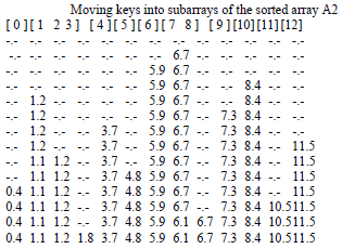
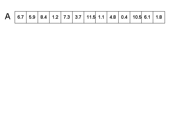
Consider a full array: A[0 to n-1] with n keys. Let i be an index of A. Sort A's keys into array A2 of equal size.
The map key function is defined as mapKey(key) = floor(K).
| A1 | 6.7 | 5.9 | 8.4 | 1.2 | 7.3 | 3.7 | 11.5 | 1.1 | 4.8 | 0.4 | 10.5 | 6.1 | 1.8 |
|---|---|---|---|---|---|---|---|---|---|---|---|---|---|
| H | 1 | 3 | 0 | 1 | 1 | 1 | 2 | 1 | 1 | 0 | 1 | 1 | |
| P | 0 | 1 | -9 | 4 | 5 | 6 | 7 | 9 | 10 | -9 | 11 | 12 | |
| L | 7 | 6 | 10 | 1 | 9 | 4 | 12 | 1 | 5 | 0 | 11 | 7 | 1 |
| A2 | 0.4 | 1.1 | 1.2 | 1.8 | 3.7 | 4.8 | 5.9 | 6.1 | 6.7 | 7.3 | 8.4 | 10.5 | 11.5 |
Pseudocode
// compute hit counts
for i = 0 to 11 // where 11 is n
{
    H[i] = 0;
}
for i = 0 to 12 // where 12 is A.length
{
    pos = MapKey(A[i]);
    H[pos] = H[pos] + 1;
}

runningTotal = 0; // compute prox map – location of start of each subarray
for i = 0 to 11
    if H[i] = 0
        P[i] = -9;
    else
        P[i] = runningTotal;
        runningTotal = runningTotal + H[i];

for i = 0 to 12 // compute location – subarray – in A2 into which each item in A is to be placed
    L[i] = P[MapKey(A[i])];

for I = 0 to 12; // sort items
    A2[I] = <empty>;
for i = 0 to 12 // insert each item into subarray beginning at start, preserving order
{
    start = L[i]; // subarray for this item begins at this location
    insertion made = false;
    for j = start to (<the end of A2 is found, and insertion not made>)
    {
        if A2[j] == <empty> // if subarray empty, just put item in first position of subarray
            A2[j] = A[i];
            insertion made = true;
        else if A[i] < A2[j] // key belongs at A2[j]
            int end = j + 1; // find end of used part of subarray – where first <empty> is
            while (A2[end] != <empty>)
                end++;
            for k = end -1 to j // move larger keys to the right 1 cell
                A2[k+1] = A2[k];
                A2[j] = A[i];
            insertion made = true; // add in new key
    }
}
Here A is the array to be sorted and the mapKey functions determines the number of subarrays to use. For example, floor(K) will simply assign as many subarrays as there are integers from the data in A. Dividing the key by a constant reduces the number of subarrays; different functions can be used to translate the range of elements in A to subarrays, such as converting the letters A–Z to 0–25 or returning the first character (0–255) for sorting strings. Subarrays are sorted as the data comes in, not after all data has been placed into the subarray, as is typical in bucket sorting.
Proxmap Searching
ProxmapSearch uses the proxMap array generated by a previously done ProxmapSort to find keys in the sorted array A2 in constant time.
Basic strategy
- Sort the keys using ProxmapSort, keeping theMapKey function, and the P and A2 arrays
- To search for a key, go to P[MapKey(k)], the start of the subarray that contains the key, if that key is in the data set
- Sequentially search the subarray; if the key is found, return it (and associated information); if find a value greater than the key, the key is not in the data set
- Computing P[MapKey(k)] takes time. If a map key that gives a good distribution of keys was used during the sort, each subarray is bounded above by a constant c, so at most c comparisons are needed to find the key or know it is not present; therefore ProxmapSearch is . If the worst map key was used, all keys are in the same subarray, so ProxmapSearch, in this worst case, will require comparisons.
Pseudocode
function mapKey(key)
  return floor(key)
  proxMap ← previously generated proxmap array of size n
  A2 ← previously sorted array of size n
function proxmap-search(key)
  for i = proxMap[mapKey(key)] to length(array)-1
    if (sortedArray[i].key == key)
      return sortedArray[i]
Analysis
Performance
Computing H, P, and L all take time. Each is computed with one pass through an array, with constant time spent at each array location.
- Worst case: MapKey places all items into one subarray, resulting in a standard insertion sort, and time of .
- Best case: MapKey delivers the same small number of items to each subarray in an order where the best case of insertion sort occurs. Each insertion sort is , c the size of the subarrays; there are p subarrays thus p * c = n, so the insertion phase take O(n); thus, ProxmapSort is .
- Average case: Each subarray is at most size c, a constant; insertion sort for each subarray is then O(c^2) at worst – a constant. (The actual time can be much better, since c items are not sorted until the last item is placed in the bucket). Total time is the number of buckets, (n/c), times = .


Having a good MapKey function is imperative for avoiding the worst case. We must know something about the distribution of the data to come up with a good key.
Optimizations
- Save time: Save the MapKey(i) values so they don't have to be recomputed (as they are in the code above)
- Save space: The proxMaps can be stored in the hitCount array,as the hit counts are not needed once the proxmap is computed; the data can be sorted back into A, instead of using A2, if one takes care to note which A values are have been sorted so far, and which not.
Comparison with other sorting algorithms
Since ProxmapSort is not a comparison sort, the Ω(n log n) lower bound is inapplicable. Its speed can be attributed to it not being comparison-based and using arrays instead of dynamically allocated objects and pointers that must be followed, such as is done with when using a binary search tree.
ProxmapSort allows for the use of ProxmapSearch. Despite the O(n) build time, ProxMapSearch makes up for it with its average access time, making it very appealing for large databases. If the data doesn't need to be updated often, the access time may make this function more favorable than other non-comparison sorting based sorts.
Generic bucket sort related to ProxmapSort
Like ProxmapSort, bucket sort generally operates on a list of n numeric inputs between zero and some maximum key or value M and divides the value range into n buckets each of size M/n. If each bucket is sorted using insertion sort, ProxmapSort and bucket sort can be shown to run in predicted linear time.[1] However, the performance of this sort degrades with clustering (or too few buckets with too many keys); if many values occur close together, they will all fall into a single bucket and performance will be severely diminished. This behavior also holds for ProxmapSort: if the buckets are too large, its performance will degrade severely.
References
- ↑ Thomas H. Cormen, Charles E. Leiserson, Ronald L. Rivest, and Clifford Stein. Introduction to Algorithms, Second Edition. MIT Press and McGraw-Hill, 2001. ISBN 0-262-03293-7. Section 8.4: Bucket sort, pp.174–177.
- Thomas A. Standish. Data Structures in Java. Addison Wesley Longman, 1998. ISBN 0-201-30564-X. Section 10.6, pp. 394–405.
- Standish, T. A.; Jacobson, N. (2005). "Using O(n) Proxmap Sort and O(1) Proxmap Search to motivate CS2 students (Part I)". ACM SIGCSE Bulletin. 37 (4). doi:10.1145/1113847.1113874.
- Standish, T. A.; Jacobson, N. (2006). "Using O(n) Proxmap Sort and O(1) Proxmap Search to motivate CS2 students, Part II". ACM SIGCSE Bulletin. 38 (2). doi:10.1145/1138403.1138427.
- Norman Jacobson "A Synopsis of ProxmapSort & ProxmapSearch" from Department of Computer Science, Donald Bren School of Information and Computer Sciences, UC Irvine.
External links
- http://www.cs.uah.edu/~rcoleman/CS221/Sorting/ProxMapSort.html
- http://www.valdosta.edu/~sfares/cs330/cs3410.a.sorting.1998.fa.html
- http://www.cs.uml.edu/~giam/91.102/Demos/ProxMapSort/ProxMapSort.c